16. Generating generalised swath profiles

Here we expain how to generate a generalised swath profile following the same algorithm described by Hergarten et al. (2014).

The outputs from the function are:

• A raster showing the extent of the swath profile, indicating the perpendicular distance of each point from the baseline (i.e. a transverse swath)
• A raster showing the extent of the swath profile, indicating the projected distance along the baseline (i.e. a longitudinal swath)
• A .txt file containing the results of the transverse swath profile. The table includes the distance of the centre of each bin across the profile, the mean and standard deviation of each bin, and the 0, 25, 50, 75 and 100 percentiles.
• A .txt file containing the results of the longitudinal swath profile. The table includes the distance of the centre of each bin along the profile, projected onto the baseline, the mean and standard deviation of each bin, and the 0, 25, 50, 75 and 100 percentiles.

In order to do so, there are a few preprocessing steps that need to be done to generate the profile baseline. These can easily be done in ArcMap, but the experienced LSDTopotools user can also write a more complex driver function to do more specialised tasks.

16.1. Preprocessing step 1: Getting your raster into the correct format

You will need to get data that you have downloaded into a format LSDTopoToolbox can understand, namely the .flt format.

To do this, read this: Converting data from ArcMap.

16.2. Preprocessing step 2: Creating the baseline

The baseline is the centre line of the swath profile. At present the SwathProfile tool uses a shapefile *.shp consisting of a series of points that define the profile. A suitable baseline can be produced in two easy steps.

1. First, create a new shapefile, setting the feature class to polyline, and create a single line feature, which will form the baseline. This can be linear, or curved, depending on what your requirements are. Next create another shapefile, this time make the feature class point.

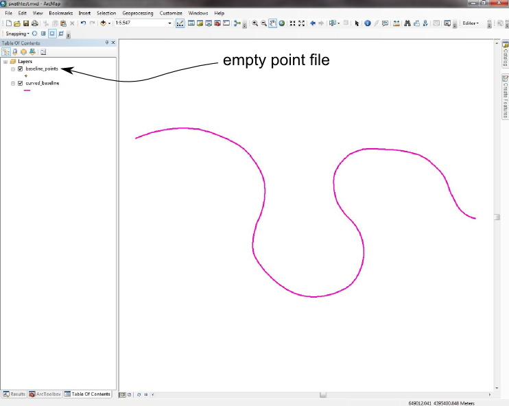
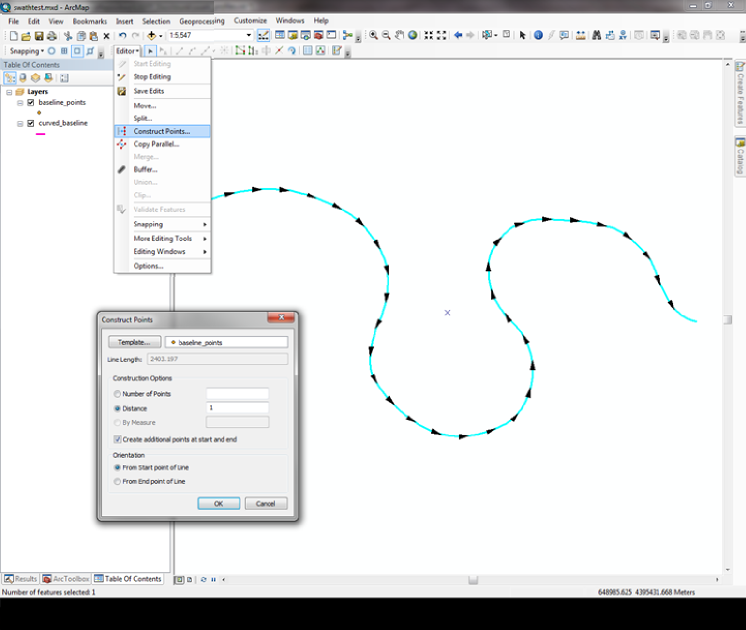
1. Start editing in ArcMap. Make the target class the new, empty point shapefile. Using the edit tool on the Editor Toolbar, select the polyline that you drew in the previous step; it should be highlighted in a light blue colour. Go to the drop-down menu on the Editor toolbar, and select “Construct Points...”. Set the template as the empty point shapefile. Set the construction option to Distance, and make the point spacing equal to the resolution of your DEM. Make sure “Create additional points at start and end” is checked. Click ok, then save your edits... you have now created the baseline file. Give yourself a pat on the back, take a deep breath and move onto the next stage...

16.3. Compiling the driver function

You will need to download all of the code. This will have a directory with the objects (their names start with LSD). Note that this tool utilises the PCL library: PCL homepage. Hopefully this is already installed on your University server (it is on the University of Edinburgh server). It probably won’t be installed on your laptop, unless you have installed it yourself at some point. This tool will not work if the PCL library is not installed!

Within the directory with the objects, there will be two additional directories:

• driver_functions
• TNT

The TNT folder contains routines for linear algebra, and it is made by NIST, you can happily do everything in LSDTopoToolbox without ever knowing anything about it, but if you want you can read what it is here: TNT homepage.

In order to compile this function, it is necessary to use cmake (version 2.8 or later). The compilation procedure is as follows:

1. First, go into the driver function folder

2. Make a new directory in this folder named build; type:

   mkdir build

   in a terminal. If you don’t know what a terminal is, read this section: Getting onto our servers using NX.

3. Move the CMakeLists_SwathProfile.txt file into the build directory. At the same time, rename this file CMakeLists.txt, so the compiler will find it. Type:

   mv CMakeLists_SwathProfile.txt build/CMakeLists.txt

4. Go into the build directory. Type:

   cmake28 .

   in the terminal. Note that the name of this directory isn’t important.

5. Next type:

   make
   

   in the terminal. This compiles the code. You will get a bunch of messages but at the end your code will have compiled.

6. All that is left to do is to move the compiled function back up into the driver_functions directory. Type:

   mv swath_profile_driver.out ..

16.4. Running the driver function

Okay, now you are ready to run the driver function. You’ll need to run the function from the directory where the compiled code is located (i.e. the driver_functions folder), but it can work on data that is located in any location.

1. You run the code with the command ./swath_profile_driver.out name_of_basline_file name_of_raster half_width_of_profile bin_width_of_profile

• The name_of_baseline_file is just the name of the shapefile created in the preprocessing step that contains the points defining the baseline.
• The name_of_raster is the PREFIX of the raster, so if your raster is called lat_26p5_flt.flt then the name_of_raster is lat_26p5_flt (that is, without the .flt at the end).
• Note that if your data is stored in a different directory, then you will need to inlude the full path name in name_of_raster and name_of_baseline_file. The output files will be saved in the same directory as the DEM.
• The half_width_of_profile is the half width of the swath (i.e. the distance from the baseline to the swath edge).
• The bin_width_of_profile is the resolution at which the profile data is condensed into a single profile. This is not the same as the raster resolution!

16.5. Program outputs

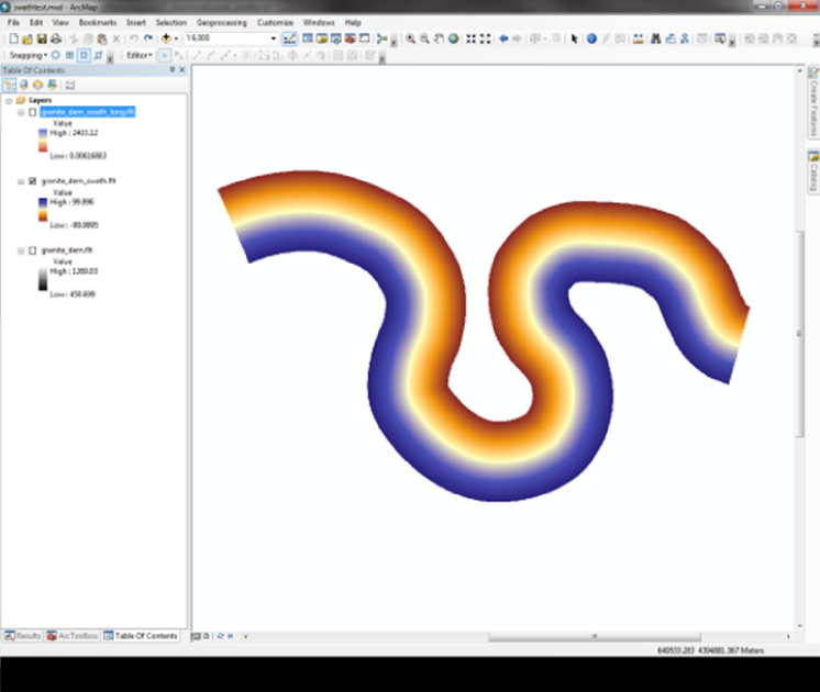
The swath_profile_driver tool creates two raster datasets, so you can check the swath templates yourself to better understand how the profiles are constructed

1. *_swath_long.flt is the longitudinal swath profile template

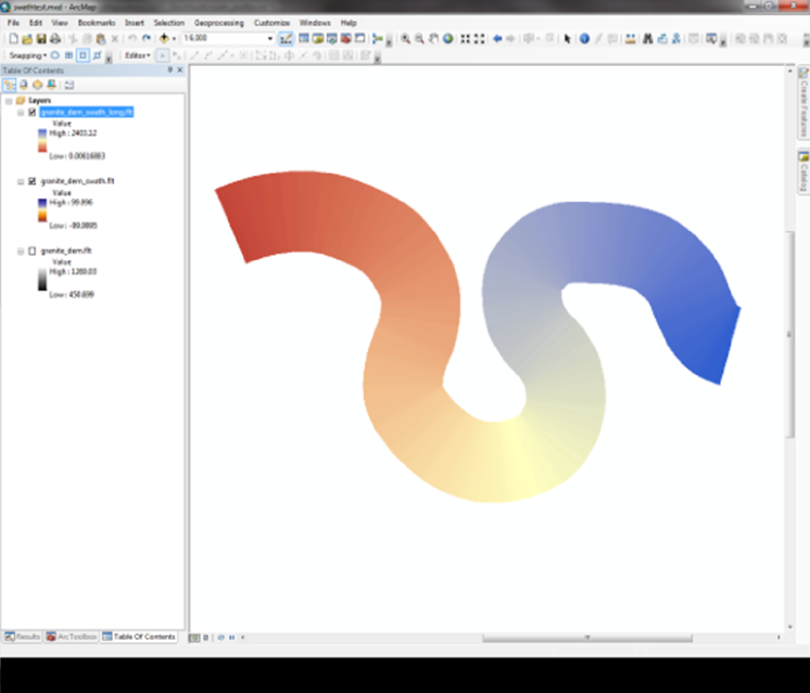
1. *_swath_trans.flt is the transverse swath profile template

There are also two .txt files, which contain the profile data -> these include the mean, standard deviation, and percentiles for each. These can be plotted using the python script plot_swath_profile.py, located in the LSDVisualisation/trunk/ directory.

16.6. Channel Long Profiles using the Swath Tools

Here another use of the swath tools feature is exploited. You can use it to automatically create long profiles along a channel using a value other than elevation, for example. (This usage is hinted at in the Hergarten et al. (2014) paper.) This application is mainly suited to where there is:

1. Expected to be some variation along channel of a certain value or other metric
2. The DEM resolution is high enough to capture lateral variations across the channel, but you are interested in the average of these metrics along the long profile.

16.6.1. Example Applications

• Channel width variation using high resolution lidar DEMs
• Sediment size distribution along channel from model output
• Erosion/deposition distribution along channel from model output
• Basin hydrology applications (water depth, velocity etc.)

You will need the driver file: longitudinal_channel_erosion_swath_profiler.cpp along with the corresponding CMake file.

There are effectively 3 supplementary files you need to perform this analysis.

• Parameter file. This takes the form of a simple text file with a column of values:
  • Terrain DEM Name (The base topography)
  • Secondary Raster/DEM file name. (This is the raster file that contains the property that varies along channel.)
  • Raster extension for the above two files (currently, both must be the same format)
  • Minslope (use 0.00001 for starters)
  • Contributing pixel threshold (for calculating the drainage network
  • Swath Half Width (see above)
  • Swath Bin Width (see above)
  • Starting Junction Number
• Terrain Raster
• Secondary Raster

These two rasters should be in the same spatial extent.

16.6.2. Example Usage

Compile the driver file using CMake. To do this, create a build folder in the driver_functions folder. Copy the file CMakeLists_Swath_long_profile_erosion.txt file into the new folder, and rename it CMakeLists.txt, as described above. Then:

cmake .
make

You now have the executable long_swath_profile_erosion.exe. It is run by giving it two arguments: the path to the parameter file and raster file (in the same directory as each other, but can be separate from the executable) and the name of the parameter file.:

./long_swath_profile_erosion.exe ./ swath_profiler_long.param

The driver file is designed to perform the whole operation in one go: Fill DEM > Extract Channel Network > Produce Channel File > Convert Channel file to X,Y Points for Swath > Create Swath Template > Perform Swath Analysis, but you may want to split it up into stages if you do not know the starting junction number where you want the profile to begin.

The driver file currently uses the longest channel in the basin (the mainstem) so check that this is what you expected. An option may become available to look at tributaries later on.

The output files are the Profile (txt) and the Swath template that was used to profile the channel. (Check that it was the spatial extent that you expected).

You can use the same visualisation script as above: plot_swath_profile.py, located in the LSDVisualisation/trunk/ directory.