8. Chi analysis, part 1: getting the channel profiles

Our chi analysis method involves two steps. The first extracts a channel profile from a DEM. This processes is separated from the rest of the chi analysis for memory management reasons: these steps involve a DEM but once they are completed chi analysis can proceed with much smaller .chan files

8.1. Quick guide

If you already know more or less what you are doing, but need a quick reminder, here are the steps involved:

1. Download your DEM.
2. Project it into a projected coordinate system (we usually use UTM).
3. Export the DEM in .flt or .bil format. See Data preparation 2: Notes for using GDAL to manipulate files for LSDTopoToolbox .
4. If the programs aren’t complied, make them with: chi_step1_write_junctions.make and chi_step2_write_channel_file.make
5. Run the program chi1_write_junctions.exe on your DEM.
6. Import the junction raster (*.JI.flt) into a GIS and pick a junction (this is easiest if you also import the stream order (*_SO.flt) and hillshade (*_HS.flt).
7. Run chi2_write_channel_file.exe to get the .chan file. Once you do this you are ready to move on to section two: running the chi analysis!

8.2. Overview

This document gives instructions on how to use the segment fitting tool for channel profile analysis developed by the Land Surface Dynamics group at the University of Edinburgh. The tool is used to examine the geometry of channels using the integral method of channel profile analysis. For background to the method, and a description of the algorithms, we refer the reader to Mudd et al. (2014). For background into the strengths of the integral method of channel profile analysis, the user should read Perron and Royden (2013, ESPL).

This document guides the user through the installation process, and explains how to use the model. You will need a c++ compiler for this tutorial. If you have no idea what a c++ compiler is, see the appendix. Visualisation of the model results is performed using Python scripts. We recommend installing Python(x,y) and running the scripts within Spyder (which is installed with Python(x,y).

Both the recommended compiler and Python(x,y) are open source: you do not need to buy any 3rd party software (e.g., Matlab) to run our topographic analysis!

8.3. Warning

This code is for research purposes and is under continuous development, so we cannot guarantee a bug-free experience!

8.4. Getting the raw DEM into the toolkit

8.4.1. Data Sources

The topographic analysis package works from a DEM. You can get these from all sorts of places. For LiDAR, two good sources are opentopography (http://www.opentopography.org/) and the U.S. Interagency Elevation Inventory (http://www.csc.noaa.gov/inventory/#). Other countries are not so progressive about releasing data but you could rummage around the links here: http://en.wikipedia.org/wiki/National_lidar_dataset. For 10m data of the United States you can go to the national map viewer (http://viewer.nationalmap.gov/viewer/). I get ASTER 30m data from the NASA’s reverb site ( http://reverb.echo.nasa.gov). One site that has filled and corrected 90-m DEMs is here: http://www.viewfinderpanoramas.org/dem3.html .

8.4.2. Getting the data into the chi profile tool

You will need to get data that you have downloaded into a format LSDTopoToolbox can understand, namely the .flt format.

To do this, read this: Converting data from ArcMap.

8.5. Compiling the two driver functions

The tools for topographic analysis are distributed as c++ source code. Before you run these tools you will have to compile them. Compiling means that you translate from source code, which looks a bit like English, to machine code, which is all 1s and 0s. To do this you use a compiler.

If you have a Linux system al you really need to do is navigate to the folder containing the source files in a terminal window. If you have a Windows computer follow the instructions in the appendix to get a compiler installed. Then you compile using a command prompt (you can find this in windows 7 by typing command prompt into the search for programs and files field in the start menu).

1. This should be fairly easy if you have your compiler installed. If you are working in the Cygwin environment (http://www.cygwin.com/) you will also need the make utility. If you are working in Linux/Unix you have almost certainly everything you need. If you are using an Apple, well I’m not sure what you do since we don’t use this operating system but I think the way to get it working is to download the Apple developer tools, install them and then open a terminal and everything should behave like a standard linux setup (Apple operating systems are built on top of linux).

2. There should be a folder with the objects named things like:

   LSDRaster.cpp, LSDFlowInfo.cpp, etc.

   There should also be two subfolders. One is the TNT subfolder which contains linear algebra routines and the other is a folder called driver_functions which contains all the drivers that are used to actually run the code. If you are missing any of this stuff go back and download what you missed.

3. Now navigate into the driver_functions folder:

   smudd@burn driver_functions $ pwd
   /home/smudd/topographic_tools/LSDRaster_chi_package/driver_functions

   It should have some driver function .cpp files as well as some .make files:

   smudd@burn driver_functions $ ls
   chi_get_profiles_driver.cpp       chi_step1_write_junctions_driver.cpp
   chi_get_profiles.make             chi_step1_write_junctions.make
   chi_m_over_n_analysis_driver.cpp  chi_step2_write_channel_file_driver.cpp
   chi_m_over_n_analysis.make        chi_step2_write_channel_file.make

4. To get the junctions, you need to compile the junction selection tool. Do this by typing:

   make -f chi_step1_write_junctions.make

   at the command line and then hitting enter.

5. Now for the next tool, which creates something called a .chan file (you don’t need to worry about what this is yet). The next tool is compiled with:

   make -f chi_step2_write_channel_file.make

6. The source code is now compiled on your system! Note: the directory structure matters. The driver functions will look for the objects (e.g., LSDRaster) and the TNT folder in its parent directory. If you’ve modified the directory structure the code will not compile.

8.6. Running the channel network extraction

The channel extraction code requires two steps. In the first step, the toolkit takes the raw DEM and prints several derived datasets from it. The main dataset used for the next step is the junction index dataset. The second step involves selecting a junction from which the chi analysis proceeds.

8.6.1. Writing junctions

1. First, create a folder for your DEM.

   For this example I am working in the Mandakini river, a tributary of the Ganga in the Indian Himalaya. Make sure both the .flt and the .hdr file are in this folder. Then you need to create a file that tells the analysis the name of the DEM and a few parameters.

   You can name this file anything you like but I have called mine chi_parameters.driver:

   smudd@burn Mandakini $ pwd
   /home/smudd/topographic_tools/test_suites/Mandakini
   
   
   smudd@burn Mandakini $ ls
   chi_parameters.driver  mandakini.flt  mandakini.hdr

2. The driver file must contain three lines. The first line is the name of the DEM without the extension. In this example the name is mandakini. The next line is a minimum slope for the fill function. The default is 0.0001. The third line is the threshold number of pixels that contribute to another pixel before that pixel is considered a channel. You can play with these numbers a bit, in this example, I have set the threshold to 300 (it is a 90m DEM so in the example the threshold drainage area is 2.5x10⁶m²). Here are the first 3 lines of the file:

   mandakini
   0.0001
   300
   

3. Once you have done this, you need to run the driver program. The driver program is called chi1_write_junctions.exe. It takes 2 arguments. The first is the path name into the folder where your data is stored, and the second is the name of the driver file. To run the program, just type the program name and then the path name and driver file name.

   The path has to end with a ‘`/`’ symbol.

   If you are working in Linux, then the program name should be proceeded with a `./` symbol. Here is a typical example:

   ./chi1_write_junctions.exe /home/smudd/topographic_tools/test_suites/Mandakini/ chi_parameters.driver

   IMPORTANT to run the code you need to be in the folder containing the .exe file, NOT the folder with the data.

   All the output from the software, however, will be printed to the data folder. That is, the software and data are kept separately.

4. In later sections you will see that the driver file has the same format for all steps, but for this step only the first three lines are read. The driver file has a bunch of parameters that are described later but there is a file in the distribution called Driver_cheat_sheet.txt that has the details of the parameter values.

5. This is going to churn away for a little while. If you have used incorrect filenames the code should tell you. The end result will be a large number of new files: The code prints

   • A filled DEM (with _fill in the filename),
   • A hillshade raster (with _HS in the filename),
   • Information about the stream orders (file with _SO in the filename),
   • A file with information about the junctions (_JI in the filename).

   So your directory will be full of files like this:

   smudd@burn Mandakini $ ls
   chi_parameters.driver  mandakini.flt     mandakini_HS.hdr  mandakini_SO.flt
   mandakini_fill.flt     mandakini.hdr     mandakini_JI.flt  mandakini_SO.hdr
   mandakini_fill.hdr     mandakini_HS.flt  mandakini_JI.hdr

   Or if you prefer a windows view

   

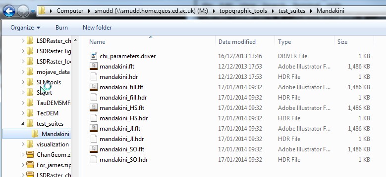
6. You will then need to load these files into ArcMap and look at them. alternative to ArcMap is Whitebox which has the advantage of being open source. QGIS is another good open source alternative to ArcMap.

7. You want to look at the channel network and junctions. So at a minimum you should import

   • the hillshade raster
   • the stream order raster (_SO in filename) and
   • the junction index raster (_JI in filename)

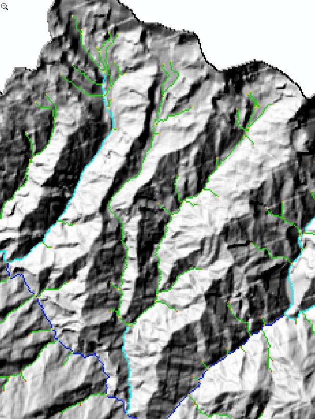
   into your preferred GIS. The stream order raster will display the channel network, with each channel having a stream order. The junction index file is the key file, you will need information from this file for the next step. In the image below, the channel network is in cool colours and the junctions are in warm colours. Each junction has a unique integer value, called the junction index.

   

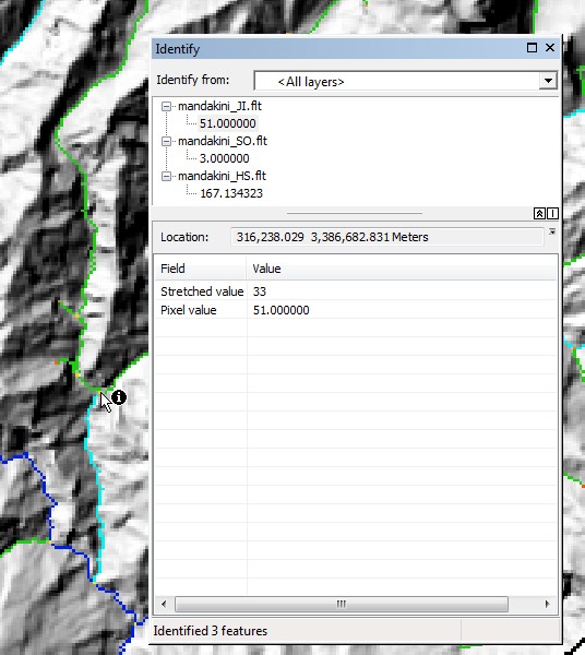
8. Now, find the part of the map where you want to do the chi analysis. You need to choose the junction at the downstream end of the channels where you will do your analysis. Use the identify tool (it looks like an `i` in a blue circle on ArcMap) to get the number of the junction that you want to use as the lowest junction in the channel network. In the below image the arrow points to junction number 51.

   

9. Each junction has one and only one receiver junction, whereas it can have multiple donor junctions. When you choose a junction, the extracted channel traces down to the node one before the receiver junction. It then traces up the channel network, following the path that leads to the node the furthest flow distance from the outlet junction. That is, when junctions are reached as the algorithm moves upstream the upstream channel is determined by flow distance not drainage area. Below we show an image of this.

8.6.2. Extracting the .chan file

1. Now that you have the junction number, you need to run the second program. Before you run this program, you need to write a file that contains the parameters for the chi analysis.

2. The first 3 lines of this file MUST be the same as the driver file in step 1. The code does not check this so you need to make sure on your own this is the case.

3. The next two rows of the driver file are the junction number from which you want to extract the network. and something that controls how the channel network is `pruned`. This is the ratio in area between the main stem and a tributary that must be exceeded for a tributary to be included in the analysis. If this number is 1 you only get the main stem. The smaller the number the more tributaries you get. A reasonable number seems to be ~0.02. Here is an example file:

   mandakini
   0.0001
   300
   51
   0.01
   

4. There can be more information in the driver file (for example, parameters for a chi analysis), but the channel network extraction program will ignore these; it only looks at the first 5 lines of the driver function.

5. From here you run the program chi2_write_channel_file.exe. You need to include the path name and the name of the chi parameter file. In Linux the program should be proceeded with ./. Here is an example:

   ./chi2_write_channel_file.exe /home/smudd/topographic_tools/test_suites/Mandakini/ chi_parameters.driver

6. This will generate several files

   • A DEM with _basin_ in the filename. Immediately before the .flt extension the junction number will also be listed. This file is a raster containing the outline of the contributing pixels to the basin drained by the extracted channel network.
   • A .chan file (with _ChanNet_ and the junction number in the filename) will be printed.
   • A .csv file. This file can be imported into ArcMap or other GIS software.

   ArcMap should be able to see the ‘.csv’ file.

   

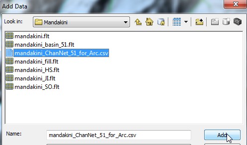
   If you load this layer and right click on it, you should be able to load the xy data

   

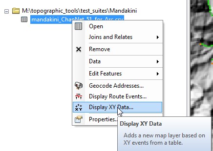
   Loading the csv file will give you a shapefile with the channel nodes, and loading the _basin_ file will give you the basin. Here is the basin and the channel for junction 51 of the Mandakini dataset

   

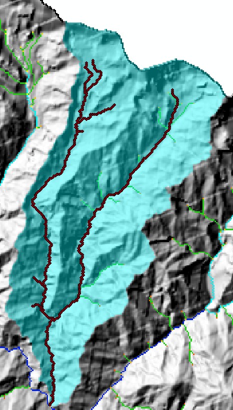
   Note how the channel extends downstream from the selected junction. It stops one node before the next junction. This way you can get an entire tributary basin that stops one node short of its confluence with the main stem channel.

8.6.3. Format of the .chan file

The segment fitting algorithm (see part 2) works on a `channel` file (we use the extension .chan to denote a channel file). The channel file starts with six lines of header information that is used to reference the channel to a DEM. If the channel is not generated from a DEM these six rows can contain placeholder values. The six rows are:

Nrows <- number of rows
Ncols <- number of columns
Xllcorner <- location in the x coordinate of the lower left corner
Yllcorner <- location in the y coordinate of the lower left corner
Node_spacing <- the spacing of nodes in the DEM
NoDataVal <- the value used to indicate no data

This header information is not used in the segment analysis; it is only preserved for channel data to have some spatial reference so that scripts can be written to merge data from the channel files with DEM data.

The rest of the channel file consists of rows with 9 columns.

• The first column is the channel number (we use c++ style zero indexing so the main stem has channel number 0).
• The second column is the channel number of the receiver channel (the channel into which this channel flows). The mainstem channel flows into itself, and currently the code can only handle simple geometries where tributaries flow into the main stem channel only, so this column is always 0.
• The third column is the node number on the receiver channel (which, recall, must be the main stem) into which the tributary flows. The main stem is defined to flow into itself. Suppose the main stem has 75 nodes. The third column would then be 74 for the main stem (because of zero indexing: the first node in the main stem channel is node 0. Nodes are organized from upstream down, so the most upstream node in the main stem channel is node zero. Suppose tributary 1 entered the main stem on the 65th node of the main stem. The third column for tributary 1 would be 64 (again, due to 0 indexing).
• The 4th column is the node index that refers back to the LSDFlowInfo object.
• The 5th column is the row in a DEM the node occupies.
• The 6th column is the column in a DEM the node occupies.
• The 7th column is the flow distance from the outlet of the node. It should be in metres.
• The 8th column is the elevation of the node. It should be in metres.
• The 9th column is the drainage area of the node. It should be in metres squared.

Many of these columns are not used in the analysis but are there to allow the user to refer the channel file back to a DEM. Columns are separated by spaces so rows will have the format:

Chan_number receiver_chan receiver_node node_index row col flow_dist elev drainage_area

Here are the first few lines of the example file (mandakini_ChanNet_51.chan):

648
587
290249.625
3352521.5
88.81413269
-9999
0 0 271 4864 70 322 71253.0625  4609.008789 3762552.25
0 0 271 4999 71 322 71164.25  4609 3770440.25
0 0 271 5140 72 322 71075.4375  4602 3778328.25
0 0 271 5288 73 322 70986.625  4596 3786216
0 0 271 5444 74 323 70861.02344  4591 3794104
0 0 271 5615 75 323 70772.21094  4574 3928199.25
0 0 271 5799 76 323 70683.39844  4571 3936087.25
0 0 271 5992 77 324 70557.79688  4565 3975527
0 0 271 6190 78 325 70432.19531  4564 3983414.75

Now that you have the .chan file you are ready to move to part 2 of the chi analysis (Chi profile analysis, part 2: constraining m/n and transforming profiles). This may have seen like quite a few steps, but once you get familiar with the workflow the entire process should take no more than a few minutes.