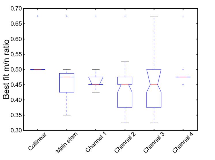
For structurally or tectonically complex landscapes, it can be difficult to constrain the  ratio.
In such cases, it is wise to perform a sensitivity analysis of the best fit ratio.
To facilitate this, we provide a python script, movern_sensitivity_driver_generation.py,
that generates a number of driver files with the parameters minimum_segment_length, sigma,
mean_skip and target_nodes that vary systematically.
ratio.
In such cases, it is wise to perform a sensitivity analysis of the best fit ratio.
To facilitate this, we provide a python script, movern_sensitivity_driver_generation.py,
that generates a number of driver files with the parameters minimum_segment_length, sigma,
mean_skip and target_nodes that vary systematically.
To run this script you will need to change the data directory and the filename of the original driver file within the script.
You will need to modify the script before you run it. On lines 41 and 43 you need to modify the data directory
and driver name of your files:
# set the directory and filename
DataDirectory =  "/home/smudd/topographic_tools/test_suites/Mandakini/"

DriverFileName = "chi_parameters.driver"
If you are running this file in Spyder from a windows machine, the path name will have slightly different formatting:
DataDirectory = "m:\\topographic_tools\\test_suites\\Mandakini\\"
Note that if you run from the command line you will need to navigate to the folder that contains the script.
The driver files will be numbered (e.g., my_driver.1.driver, my_driver.2.driver, etc.):
smudd@burn Mandakini $ ls *.driver
chi_parameters.1.driver
chi_parameters.2.driver
chi_parameters.driver
You can run these with:
./chi_m_over_n_analysis.exe /home/smudd/topographic_tools/test_suites/Mandakini/ my_driver.1.driver
Or if you want to run them with no hangup and nice:
nohup nice ./chi_m_over_n_analysis.exe /home/smudd/topographic_tools/test_suites/Mandakini/ my_driver.1.driver &
And then just keep running them in succession until you use up all of your CPUs (luckily at Edinburgh we have quite a few)!
We have also written an additional python script called Run_drivers_for_mn.py which simply looks for all the drivers in folder
and sends them to your server. Once again, you’ll need to modify this python script before you run it in order to
give the script the correct data directory. In this case the relevant line is line 18:
DataDirectory = "/home/smudd/topographic_tools/test_suites/Mandakini/"
You can run it from command line with:
python Run_drivers_for_mn.py
Again, you’ll need to be in the directory holding this file to run it (but it doesn’t have to be in the same directory as the data).
Warning: this will send all drivers to your servers to be run, so if you generated 1000 drivers, then 1000 jobs will be
sent to the server. Use with caution!
 values chi_visualisation.py
 ) space.
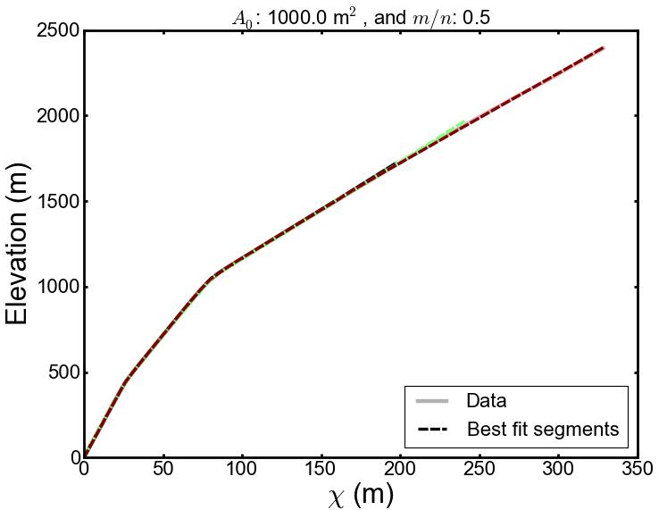
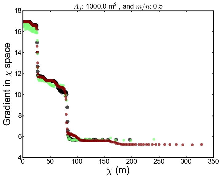
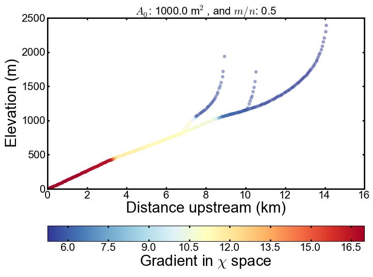
The transformation involves integrating drainage area along the length of the channel,
so that comparisons of channel steepness can be made for chanels of different drainage area.
) space.
The transformation involves integrating drainage area along the length of the channel,
so that comparisons of channel steepness can be made for chanels of different drainage area. in the
  (from n_iterations iterations)
for each tested
(from n_iterations iterations)
for each tested  value for the node.
 value for the node.
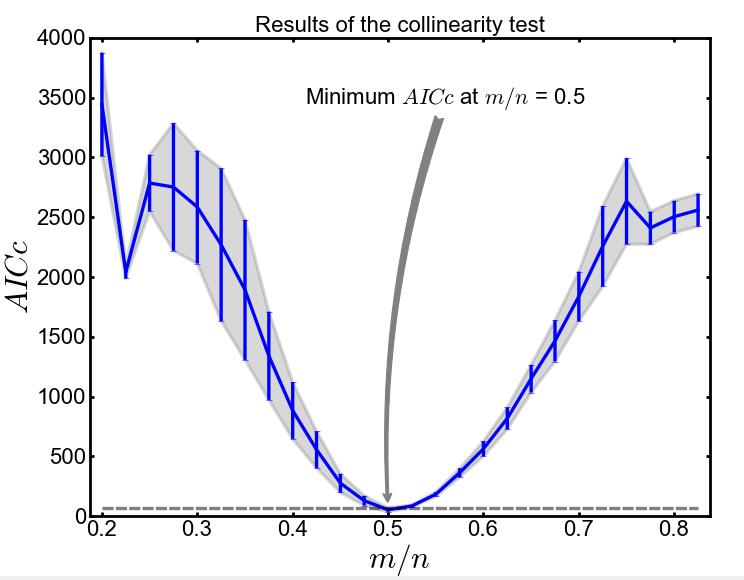