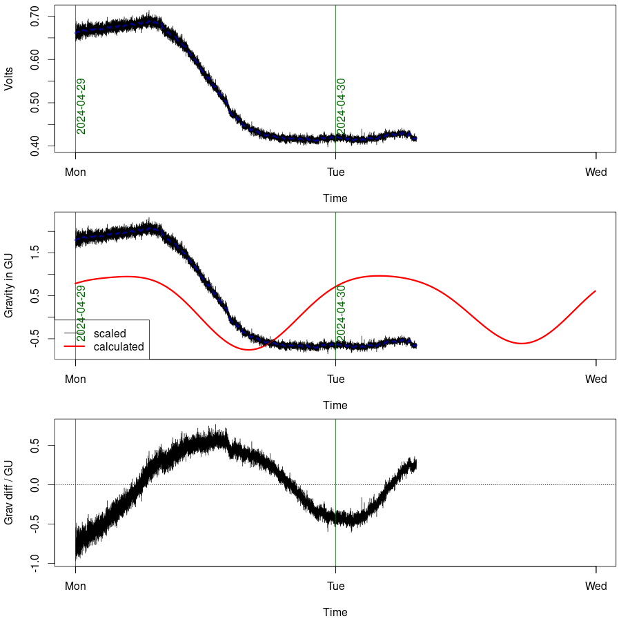
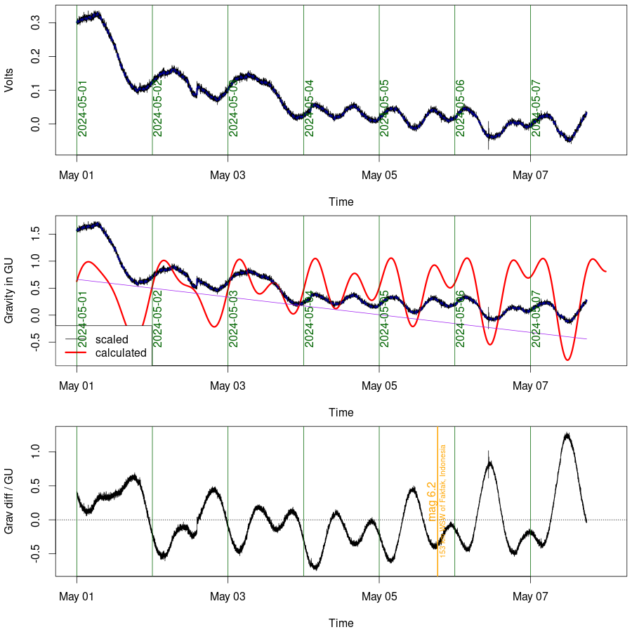
In the figures below, the top graph is the voltage at the beam galvanometer of a Lacoste-Romberg gravity meter. If everything is working properly the plot should be updated every five minutes. The data are recorded at a rate of one point every 5 seconds. The red curve in the centre graph is the theoretical gravity tide, calculated using the venerable formulas of Longman (1959); the voltage is scaled and shifted so it can be easily compared. The bottom graph shows the difference between the theory and the scaled measurement, with a linear drift included. An estimate of the linear drift is shown in purple on the middle graph. The shifting and scaling doesn't work well when there has been a break in the data, e.g. when I have had to re-balance the gravimeter, or when it has been away from the lab doing fieldwork. The orange markers are earthquakes of magnitude greater than 5.6 as reported by the USGS
Plots were a bit weird in June 2023 because I had the instrument that usually produces them at my house for field testing purposes. The plots came from an instrument I found in the back of a cupboard and assumed for many years to be dead. Reports of its deadness appear to be at least a little exaggerated. From July 2023 until October 2023 the usual the usual instrument was back on duty, but it is currenty at ZLS for a service; the dodgy instrument is currently on duty.


All of these models attempt to interpret some measurements of Bouguer anomaly in terms of density contrasts in the underlying rocks. All also make the very simple assumption that the density contrasts vary only with depth and along the survey line. They are therefore appropriate for a situation where a survey line crosses known structures (faults, dykes, railway tunnels etc.) at right-angles. All models are (c) me and released under the GNU GPL.
All models are written in R , so you need to download R and install it. It is free and installs easily on Windows, MacOSX and Linux (where it is probably packaged for your favourite distribution). R is installed already on most School of GeoSciences computers.
Ideally, you should be able to run the models by double-clicking on them, or by typing (e.g.) ./gravls.R at the Linux shell prompt. But you may have to set things up first.
All models have a variety of parameters which you can enter and a data panel into which you can cut-and-paste two columns of data. These should be distance in metres and Bouguer anomaly in gu. The program will plot your data and attempt to fit a model to it.
With gravls.R and gravts.R you will need to set the number of faults or of line sources by hand. The program merely moves these about in its attempt to fit your data. It will only succeed if your initial guess is good enough.
With grav2d.R, the main things you have control over are the resolution of the model (how many grid boxes it uses), the width and depth over which the density contrasts extend, and the damping used by the inversion.
We use python as a teaching language on the geophysics degrees. I am gradually re-writing the gravity models in python, partly to make them easier for the students to run and partly in the fond hope that they might look at the code to see how it works. To run these, you will need to have the python modules numpy and matplotlib installed. On Linux, you should be able to give yourself execute permission and then run the program in the same way as for the R version. On Windows you should be able to run the program from within your favourite IDE (e.g. Spyder) or right-click it and choose "open with" ==> "python".